cs188-note14
Non-Deterministic Search
我们将要解决带有不确定性的问题,也就要用到下面的模型,Markov decision processes,也就是MDPs.
Markov Decision Processes
下面介绍几个属性:
- A set of states S. 也就是States
- A set of actions A. 也就是Actions
- A start state
- Possibly one or more terminal states
- Possibly a discount factor $γ$.
- A transition function T (s, a, s′). it’s a probability function which represents the probability that an agent taking an action a ∈ A from a state s ∈ S ends up in a state s′ ∈ S.
- A reward function R(s, a, s′). 类似前面的note中提到的evaluate function
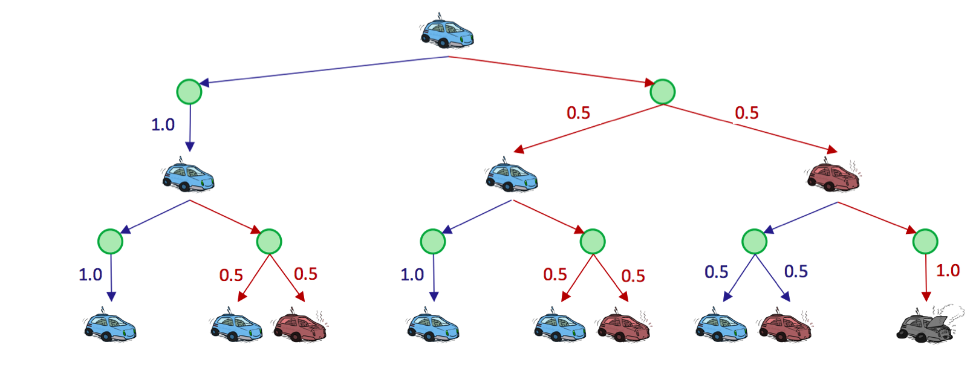
Uncertainty is modeled in these search trees with Q-states, also known as action states
The Qstate represented by having taken action a from state s is notated as the tuple (s, a).
绿色节点便是Q-states.where an action has been taken from a state but has yet to be resolved into a successor state.
Finite Horizons and Discounting
it could routinely choose a = slow at every timestep forever, safely and effectively obtaining infinite reward without any risk of overheating.
Finite Horizons:相当于一个lifetime,在它们被自动终止前来获得尽可能多的reward
Discounting factors(model an exponential decay in the value of rewards over time)
Concretely, with a discount factor of γ, taking action at from state st at timestep t and ending up in state st+1 results in a reward of γtR(st, at, st+1) instead of just R(st, at, st+1).
instead of maximizing the additive utility
\[U([s_0, a_0, s_1, a_1, s_2, \ldots]) = R(s_0, a_0, s_1) + R(s_1, a_1, s_2) + R(s_2, a_2, s_3) + \ldots\]we attempt to maximize discounted utility
\[U([s_0, a_0, s_1, a_1, s_2, \ldots]) = R(s_0, a_0, s_1) + \gamma R(s_1, a_1, s_2) + \gamma^2 R(s_2, a_2, s_3) + \ldots\]| 上面的式子看起来和几何级数差不多,只要 | γ | < 1,则可以确认finite-valued成立 |
Markovianess
达成Markovianess,需要满足Markov property,也就是无记忆性。
\[P(Xn+1=x∣Xn=y,Xn−1=z,…,X0=w)=P(Xn+1=x∣Xn=y)\] \[T (s, a, s′) = P(s′|s, a)\]Solving Markov Decision Processes
An optimal policy is one that if followed by the implementing agent, will yield the maximum expected total reward or utility
The Bellman Equation
先引入两个新变量
- The optimal value of a state s, $U^∗(s)$: 最优的agent所获得的期望值,与$V^∗(s)$同
- The optimal value of a Q-state (s, a), $Q^∗(s, a)$: 从s开始,取a并采取最优行动后获得的效用的预期值。
The Bellman Equation的定义如下
\[U^*(s) = \max_a \sum_{s'} T(s, a, s') \left[ R(s, a, s') + \gamma U^*(s') \right]\]the equation for the optimal value of a Q-state(optimal Q-state)
\[Q^*(s, a) = \sum_{s'} T(s, a, s') \left[ R(s, a, s') + \gamma U^*(s') \right]\]Note that this second definition allows us to reexpress the Bellman equation as
\[U^*(s) = \max_a Q^*(s, a)\]最有条件则相当于$∀s ∈ S, U(s) = U^∗(s)$
Value Iteration
Value iteration is a dynamic programming algorithm that uses an iteratively longer time limit to compute time-limited values until convergence (that is, until the U values are the same for each state as they were in the past iteration
- ∀s ∈ S, initialize $U_0(s)$ = 0. 0 timesteps means no actions can be taken before termination, and so no rewards can be acquired.
- Repeat the following update rule until convergence
In essence, we use computed solutions to subproblems (all the Uk(s)) to iteratively build up solutions to larger subproblems (all the Uk+1(s)); this is what makes value iteration a dynamic programming algorithm.
为了方便,我们可以将上面的方程速记一下:
\[U_{k+1} ← BU_k\]B is called the Bellman operator,The Bellman operator is a contraction by γ.
为了证明上面的,我们需要下面的不等式
\[\left| \max_z f(z) - \max_z h(z) \right| \leq \max_z \left| f(z) - h(z) \right|\]Policy Extraction
\[\forall s \in S, \quad \pi^*(s) = \arg\max_a Q^*(s, a) = \arg\max_a \sum_{s'} T(s, a, s') \left[ R(s, a, s') + \gamma U^*(s') \right]\]Q-Value Iteration
\[Q^{k+1}(s, a) \leftarrow \sum_{s'} T(s, a, s') \left[ R(s, a, s') + \gamma \max_{a'} Q^k(s', a') \right]\]Policy Iteration
- Define an initial policy. This can be arbitrary, but policy iteration will converge faster the closer the initial policy is to the eventual optimal policy.
- Repeat the following until convergence: • Evaluate the current policy with policy evaluation. For a policy π, policy evaluation means computing Uπ (s) for all states s, where Uπ (s) is expected utility of starting in state s when following π:
1
 Define the policy at iteration i of policy iteration as πi. Since we are fixing a single action for each state, we no longer need the max operator which effectively leaves us with a system of |S| equations generated by the above rule. Each Uπi(s) can then be computed by simply solving this system. Alternatively, we can also compute Uπi(s) by using the following update rule until convergence, just like in value iteration:
1
2
3
However, this second method is typically slower in practice.

• Once we’ve evaluated the current policy, use policy improvement to generate a better policy. Policy improvement uses policy extraction on the values of states generated by policy evaluation to generate this new and improved policy:
1
If πi+1 = πi, the algorithm has converged, and we can conclude that $π_{i+1} = π_i = π_∗$.
Summary
The material presented above has much opportunity for confusion. We covered value iteration, policy iteration, policy extraction, and policy evaluation, all of which look similar, using the Bellman equation with subtle variation. Below is a summary of the purpose of each algorithm:
- Value iteration: Used for computing the optimal values of states, by iterative updates until convergence.
- Policy evaluation: Used for computing the values of states under a specific policy.
- Policy extraction: Used for determining a policy given some state value function. If the state values are optimal, this policy will be optimal. This method is used after running value iteration, to compute an optimal policy from the optimal state values; or as a subroutine in policy iteration, to compute the best policy for the currently estimated state values.
- Policy iteration: A technique that encapsulates both policy evaluation and policy extraction and is used for iterative convergence to an optimal policy. It tends to outperform value iteration, by virtue of the fact that policies usually converge much faster than the values of states.
